GeoScopes

In order to run spatially-explicit simulations, we have to have a way to define “space”. Which places are included in our simulation? In epymorph, this question is answered by the GeoScope.

Unlike agent-based models which typically track individuals moving about in continuous space, we divide the world into a finite number of locations. Every person in the system is in exactly one location at any point in time. And every location is treated as a pool of individuals who all have an equal likelihood of interacting with each other (sometimes referred to as being “well-mixed”).

For example if our GeoScope includes all of the counties in Arizona, a person can be in Maricopa County and interact with other people in Maricopa County. Due to the mechanics of our movement model, they may in the next day move to Yavapai County and thus come into contact with other people in Yavapai County.

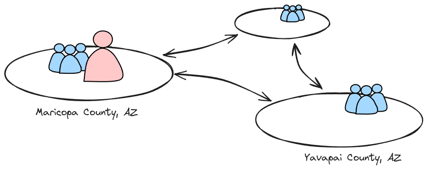
We often use the term node to refer to locations in a GeoScope, borrowing terminology from graph theory which composes graphs out of nodes and edges. You could imagine our geo nodes being connected by edges which allow individuals to “pop” between them.

GeoScopes themselves don’t contain very much information. A GeoScope contains only three things:

how many nodes it includes,
a unique identifier for each node, and
the canonical ordering of those nodes.

GeoScopes do not include information about things like how many square miles in area are each of the nodes, how can we draw a map of the nodes, or which nodes share borders. For concerns like that, we use GeoScopes like a key to access data which is associated with the geography. Thus geo nodes and various data attributes associated with those nodes are different things. This keeps epymorph’s geography systems as flexible as possible.

To underscore that, let’s look at how epymorph models geography which is entirely arbitrary – that is, it doesn’t mirror the real world at all!

Custom scopes

CustomScopes give you the most flexibility in representing geography.

from epymorph.kit import *

scope = CustomScope(["A", "B", "C"])

That’s all I need to define a geo scope containing three fictional locations, known as A, B, and C. Notice that I have specified all three things mentioned above: the number of nodes (3), a unique identifier for each, and the canonical order (the order listed). We could ask scope to repeat that information if we didn’t know for sure:

scope.nodes

scope.node_ids

array(['A', 'B', 'C'], dtype='<U1')

scope.labels  # CustomScopes use the node IDs as labels

array(['A', 'B', 'C'], dtype='<U1')

Of course it’s going to be impossible to automatically draw maps or load demographic data for fictional places. Some parts of epymorph will not work with custom scopes. But you can use them to run simulations, you would just have to provide (or invent) the required data yourself.

United States geography

Because many modelers will want to run simulations that reflect the real world, epymorph includes a system of CensusScopes that provide additional functionality. These are so called because they match the system of geographic delineations defined by the US Census Bureau. Specifically: states, counties, census tracts, and census block groups (CBGs). (Note that when we talk about states we really mean US States and state-equivalents, which include territories like Puerto Rico; when we talk about counties we mean counties and county-equivalents, which include county-like structures which are not legally counties. Geography is complicated so it’s helpful to be able to simplify!)

Note: epymorph’s supported States

epymorph omits some territories (state-equivalents) from the CensusScope system. This design decision was made to align with one of our primary data sources, the US Census Bureau’s American Community Survey (ACS). So when you ask epymorph for “all” states, you get the fifty States, the District of Columbia, and Puerto Rico — all of which are included in ACS results. But know that this does leave out four territories: American Samoa, Guam, the Northern Mariana Islands, and the US Virgin Islands.

Census delineations are convenient for a few reasons:

They are perfectly nested; the United States is composed entirely of states, each state is composed entirely of counties, each county of tracts, and each tract of CBGs.
They are regular; every square inch of the US belongs to exactly one of each, and there’s no weird overlaps or counties which belong to two states, etc.
The Census Bureau publishes data organized using these delineations, as do many other data sources.
The Census Bureau publishes files which define the shapes of the delineations (so we can draw them).
Each has a unique ID (a.k.a. FIPS code or GEOID), and the IDs themselves have a convenient nested structure.

(A wealth of additional information on Census geography can be found on their website.)

We often refer to the “levels” of this hierarchy as granularity, because states tend to be large (coarse granularity) and CBGs tend to be small (fine granularity). epymorph assumes when you want to define a geo scope, that all of your nodes are going to be the same granularity.

Note

There is actually one step smaller than block groups — “blocks”. We omitted block granularity scopes to keep things simple. It is difficult to find much high-quality data at the scale of individual blocks, so they’re not very useful to us.

Constructing CensusScopes

Now some examples. GeoScopes which reflect the US Census geography all extend from base class CensusScope. Each subclass represents a level of granularity, so there are StateScope, CountyScope, TractScope, and BlockGroupScope to choose from.

Creating a scope with all of the counties in Arizona looks like this:

scope = CountyScope.in_states(["AZ"], year=2020)

Now we can get the list of the 15 counties’ FIPS codes:

scope.node_ids

array(['04001', '04003', '04005', '04007', '04009', '04011', '04012',
       '04013', '04015', '04017', '04019', '04021', '04023', '04025',
       '04027'], dtype='<U5')

And the county labels:

scope.labels  # CensusScopes have friendlier labels

array(['Apache, AZ', 'Cochise, AZ', 'Coconino, AZ', 'Gila, AZ',
       'Graham, AZ', 'Greenlee, AZ', 'La Paz, AZ', 'Maricopa, AZ',
       'Mohave, AZ', 'Navajo, AZ', 'Pima, AZ', 'Pinal, AZ',
       'Santa Cruz, AZ', 'Yavapai, AZ', 'Yuma, AZ'], dtype='<U14')

If I just wanted a few specific counties, I would construct my scope like this:

scope = CountyScope.in_counties(["Maricopa, AZ", "Coconino, AZ"], year=2020)

scope.labels

array(['Coconino, AZ', 'Maricopa, AZ'], dtype='<U12')

There are many ways to construct scopes, but the pattern is the same. First I decide the granularity at which I want to model; StateScope/CountyScope/etc. Then I decide which of those places I want; .in_states()/.in_counties()/etc. Finally I decide which geographic year I want.

Census delineation year

This may seem strange at first, but Census delineations can and do change from year to year. The set of states in the US is very stable — the last state to enter the Union was Hawaii in 1959. But counties have changed in 2022, 2020, 2015, 2014, and so on, usually only a few at a time. Tracts and CBGs change much more often. Counting CBGs (in the states that epymorph supports), in 2019 there were 220,333 CBGs and in 2020 there were 242,335. So the year really matters! The year is sometimes referred to as the “vintage”, especially when data is being coded to a particular year’s geography. If I’m loading data expecting to find 2022 counties but the data uses 2020 counties I might not get all of the data I’m expecting.

Census node IDs

Internally, CensusScope instances always identify nodes using numerical codes which are sometimes called FIPS codes (for states or counties) or geo IDs (for smaller granularities). When constructing a CensusScope instance you have more options though. States can be identified by their full name ("Arizona"), postal code ("AZ"), or FIPS code ("04"). Counties can be identified by their full name and state postal code ("Maricopa, AZ") or FIPS code ("04013"). Tracts and CBGs can only be identified numerically however. When constructing a scope, you must be consistent in the type of identifier you use but you’re free to choose whichever is most convenient.

The system of Census delineation numerical codes have some neat properties which are helpful to understand. First: each granularity is represented by a fixed number of digits. Second: lower granularities are always prefixed by the code of the parent granularity. The table contains some examples to illustrate the point (prefix digits in bold):

Granularity	Number of Digits	Example Code
state	2	04 Arizona
county	5	04013 Maricopa County, Arizona
tract	11	04013010102 Census Tract 101.02, Maricopa County, Arizona
CBG	12	040130101021 Block Group 1, Census Tract 101.02, Maricopa County, Arizona

And even though these codes use only numerical digits, they are not numbers! Leading zero digits are significant, so treat them as strings.

Census utilities

Although not necessary in typical epymorph usage, there are some additional features that can come in handy.

Shift granularity

A CensusScope using one granularity can be “shifted” up or down the granularity scale using .raise_granularity() and .lower_granularity(). For example:

# Start with all counties in Arizona
counties_in_az = CountyScope.in_states(["AZ"], year=2020)

# "Down-shift" to all tracts in Arizona
tracts_in_az = counties_in_az.lower_granularity()

tracts_in_az.node_ids

array(['04001942600', '04001942700', '04001944000', ..., '04027980004',
       '04027980005', '04027980006'], dtype='<U11')

Be aware that when shifting up, you may effectively broaden your selection:

# Start with just Maricopa, AZ
one_county_az = CountyScope.in_counties(["Maricopa, AZ"], year=2020)

# Shift up to state
az_state = one_county_az.raise_granularity()

az_state.node_ids

array(['04'], dtype='<U2')

# Shift back to county
counties_again = az_state.lower_granularity()

counties_again.node_ids  # oh now we've got *all* AZ counties!

array(['04001', '04003', '04005', '04007', '04009', '04011', '04012',
       '04013', '04015', '04017', '04019', '04021', '04023', '04025',
       '04027'], dtype='<U5')

Name/ID mappings

For states and counties it may be useful to have dictionaries which represent the mappings between names and FIPS codes, and so on. As a convenience, epymorph does make those available. For instance:

from epymorph.geography.us_tiger import get_states

get_states(year=2020).state_fips_to_name
# (or postal code)   .state_fips_to_code

{'01': 'Alabama',
 '02': 'Alaska',
 '04': 'Arizona',
 '05': 'Arkansas',
 '06': 'California',
 '08': 'Colorado',
 '09': 'Connecticut',
 '10': 'Delaware',
 '11': 'District of Columbia',
 '12': 'Florida',
 ...
}

And:

from epymorph.geography.us_tiger import get_counties

get_counties(year=2020).county_fips_to_name

{'01001': 'Autauga, AL',
 '01003': 'Baldwin, AL',
 '01005': 'Barbour, AL',
 '01007': 'Bibb, AL',
 '01009': 'Blount, AL',
 '01011': 'Bullock, AL',
 '01013': 'Butler, AL',
 '01015': 'Calhoun, AL',
 '01017': 'Chambers, AL',
 '01019': 'Cherokee, AL',
 ...
}

GeoDataFrames

If you would like to work with the GeoDataFrames, there are utility functions to do that as well.

import geopandas as gpd

from epymorph.geography.us_tiger import get_states_geo

# Load the geopandas GeoDataFrame for all states:
states_gdf = get_states_geo(year=2020)
states_gdf.head()

	GEOID	STUSPS	NAME	ALAND	INTPTLAT	INTPTLON	geometry
0	54	WV	West Virginia	62266296765	+38.6472854	-080.6183274	POLYGON ((-81.74725 39.09538, -81.74635 39.096...
1	12	FL	Florida	138958484319	+28.3989775	-082.5143005	MULTIPOLYGON (((-86.39964 30.22696, -86.40262 ...
2	17	IL	Illinois	143778461053	+40.1028754	-089.1526108	POLYGON ((-91.18529 40.63780, -91.17510 40.643...
3	27	MN	Minnesota	206232157570	+46.3159573	-094.1996043	POLYGON ((-96.78438 46.63050, -96.78434 46.630...
4	24	MD	Maryland	25151895765	+38.9466584	-076.6744939	POLYGON ((-77.45881 39.22027, -77.45866 39.220...

# Filter the previous GDF using the states in a scope:
scope = StateScope.in_states(["AZ", "CO", "NM", "UT"], year=2020)
scope_gdf = gpd.GeoDataFrame(states_gdf[states_gdf["GEOID"].isin(scope.node_ids)])
scope_gdf.head()

	GEOID	STUSPS	NAME	ALAND	INTPTLAT	INTPTLON	geometry
12	35	NM	New Mexico	314198560935	+34.4346843	-106.1316181	POLYGON ((-106.00632 36.99527, -106.00531 36.9...
23	49	UT	Utah	213355058738	+39.3349925	-111.6563326	POLYGON ((-114.04703 39.90610, -114.04702 39.9...
26	08	CO	Colorado	268418746964	+38.9937669	-105.5087122	POLYGON ((-109.05095 40.22265, -109.05097 40.2...
55	04	AZ	Arizona	294360991275	+34.2039362	-111.6063449	POLYGON ((-114.51684 33.02789, -114.51699 33.0...

See:

The rest of the world…

Earth is a pretty big place and we appreciate that there is a lot of important and exciting epidemiology happening in many, many places outside the United States. Ultimately we would love to include geographic systems which describe the rest of the world in ways that are useful in those places. (Maybe you can help us with that!) For now CustomScope is designed to be the fallback for geographies that aren’t currently modeled in epymorph. Please do let us know what we can do to support the kind of modeling work you are interested in doing.