Getting Started

Let’s start by looking at a very simple epymorph simulation. Our focus is just to get something running, so don’t worry if there are unfamiliar concepts. We’ll learn more about all of that later.

A first example

Run this code however you like. You could copy the code into a Python script file and execute it. Or paste it into a Jupyter code cell and run that. Just make sure that the environment that has epymorph installed is active as is appropriate. In any case you should see an output like the one below.

from epymorph.kit import *
from epymorph.adrio import us_tiger


rume = SingleStrataRUME.build(
    ipm=ipm.SIRS(),
    mm=mm.Centroids(),
    init=init.SingleLocation(location=0, seed_size=100),
    scope=StateScope.in_states(["AZ", "CO", "NM", "UT"], year=2020),
    time_frame=TimeFrame.rangex("2020-01-01", "2021-01-01"),
    params={
        "beta": 0.3,
        "gamma": 1/5,
        "xi": 1/90,
        "population": [
            7_151_502, # Arizona
            5_773_714, # Colorado
            2_117_522, # New Mexico
            3_271_616, # Utah
        ],
        "centroid": us_tiger.InternalPoint(),
    },
)

sim = BasicSimulator(rume)
output = sim.run(rng_factory=default_rng(42))

output.plot.line(
    geo=output.rume.scope.select.all(),
    time=output.rume.time_frame.select.all(),
    quantity=output.rume.ipm.select.compartments("I"),
)

Explanation

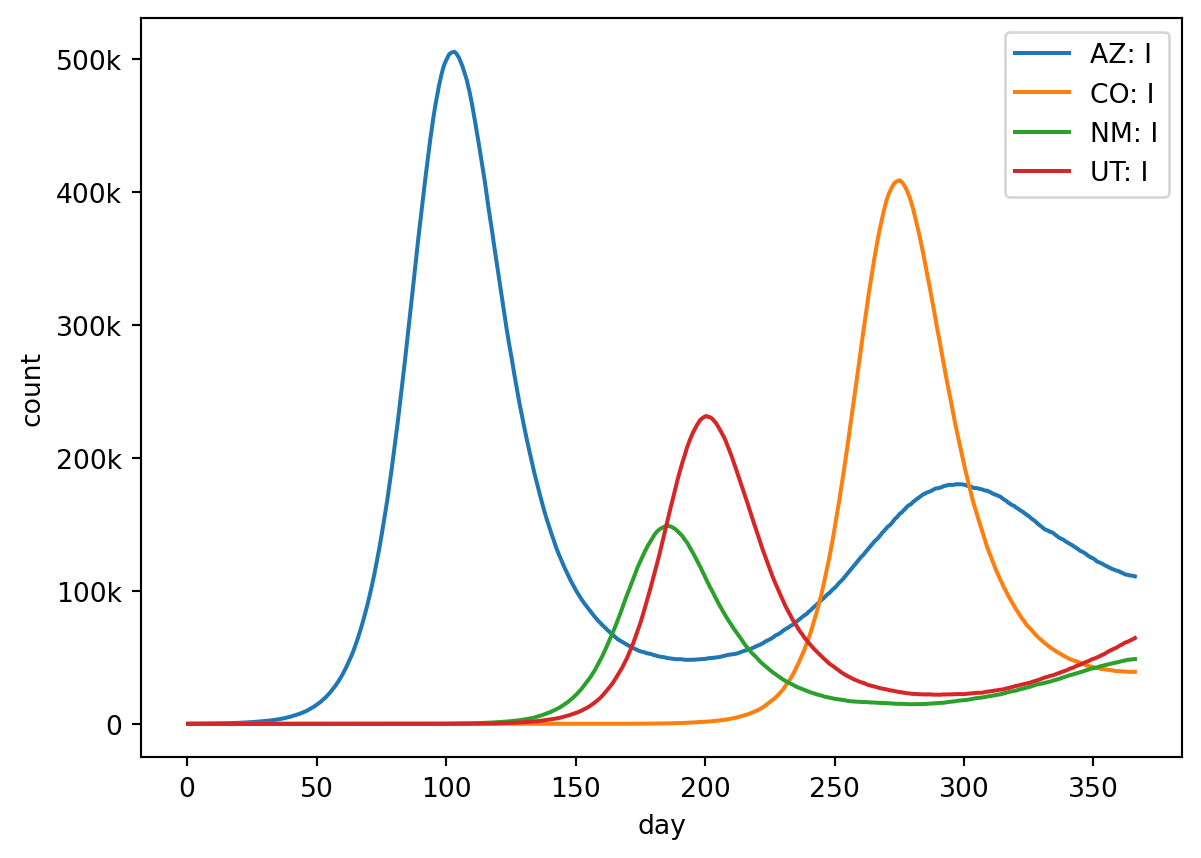
Nice! We just ran a spatially-explicit simulation of an infectious pathogen across four US States for the year 2020. Then we plotted the results, looking at how the number of infected individuals (the “I” compartment) changes over time in each location.

To do so, we followed these steps:

1. Import the required bits from epymorph.
2. Construct a Runnable Modeling Experiment (or RUME). This combines the following components:
   1. A compartmental model describing the pathogen. This is called the IPM.
   2. A movement model describing how people move between locations; MM for short.
   3. The initial conditions; how many people are infected when the simulation starts? This logic is provided by an initializer.
   4. A geographic model that we would like to simulate; what are the locations? This is called the geo scope.
   5. A time frame we would like to simulate.
   6. Values for the parameters of our models.
3. Construct a BasicSimulator using the RUME.
4. Run it once and save its output.
5. Use the output to display a line plot.

For this example I took a few short-cuts for the sake of simplicity, and these are worth pointing out.

First, notice I hard-coded population values for each of the states. It would be awfully tedious if we had to look up this info every time. Later we’ll see how epymorph can fetch this data for us dynamically.

Second, I set a seeded random number generator for the call to run(). This is just so that I get consistent results. epymorph is designed to be stochastic in nature. By default, each run produces random variations in the output. But sometimes (like when writing documentation) you want to control that randomness by setting a seed. So while it’s an option it isn’t necessary, and it may be counterproductive for your use-case.

epymorph.kit

Lastly, a word about imports. As a convenience feature, epymorph includes the epymorph.kit package which you can use in a star-import. Like a “starter kit”, this is designed to give you quick acccess to the most-commonly-used classes and methods in epymorph. Things like SingleStrataRUME (for describing experiments) and ipm (our package of built-in IPMs) are made available from that import. (See the full list here.)

However you can always import the classes directly if you prefer to have full control over the things in your namespace. For example without the kit import, the above imports might look like this:

from epymorph.adrio import us_tiger
from epymorph.data import ipm, mm
from epymorph.geography.us_census import StateScope
import epymorph.initializer as init
from epymorph.rume import SingleStrataRUME
from epymorph.simulation import default_rng
from epymorph.simulator.basic.basic_simulator import BasicSimulator
from epymorph.time import TimeFrame