Estimating space- and time-varying transmission rate from data

Scenario

It is common that we want to account for and quanitfy heterogeneity in transmission rates among localities to better understand the regional picture of pathogen spread. Therefore, we may have a spatial model with multiple nodes, and we want to understand from data how the transmission rate varies among localities. We may also want to quantify this spatial heterogeneity while also accounting for host movement among localities. In epymorph, we have built convenient parameter estimation functionality that allows us to estimate location- and time-varying parameters. In this scenario, we will explore how to set up the model and particle filter simulation, and we will demonstrate the critical role of the particle filter resampling protocol for optimizing the power of our analysis.

Exercise 1

We will first demonstrate why the single-node particle filter from the ealier vignette is insufficient for higher-dimentional problems. First, we will develop a multi-node simulation that does not include the effects of movement.

import numpy as np

from epymorph.kit import *
from epymorph.adrio import acs5
from epymorph.initializer import Proportional

• Construct a RUME with a scope consisting of four States, but assume that there is no movement between the states. Essentially, this simulates four independent populations. Use an SIRH IPM. In each State, initialize a small fraction initially infectious. Run for 26 weeks.

states = ["AZ", "CO", "NM", "UT"]

rume = SingleStrataRUME.build(
    ipm=ipm.SIRH(),
    mm=mm.No(),
    scope=StateScope.in_states(states, year=2015),
    init=Proportional(
        ratios=np.broadcast_to(
            np.array([9999, 1, 0, 0], dtype=np.int64), shape=(len(states), 4)
        )
    ),
    time_frame=TimeFrame.of("2022-09-15", 7 * 26 + 1),
    params={
        "beta": 0.3,  # Placeholder value
        "gamma": 0.2,
        "xi": 1 / 365,
        "hospitalization_prob": 200 / 100_000,
        "hospitalization_duration": 5.0,
        "population": acs5.Population(),
    },
)

• Specify the parameters to be estimated, modeling the beta in each state using geometric Brownian motion with a uniform initial distribution.

from epymorph.parameter_fitting.distribution import Uniform
from epymorph.parameter_fitting.utils.parameter_estimation import EstimateParameters
from epymorph.parameter_fitting.dynamics import GeometricBrownianMotion

params_space = {
    "beta": EstimateParameters.TimeVarying(
        distribution=Uniform(a=0.1, b=0.8),
        dynamics=GeometricBrownianMotion(volatility=0.1),
    ),
}

• Create the observations object using CDC weekly hospitalization data in each state.

from epymorph.adrio.cdc import InfluenzaHospitalizationSumState
from epymorph.parameter_fitting.likelihood import Poisson
from epymorph.parameter_fitting.utils.observations import ModelLink, Observations
from epymorph.time import EveryNDays

observations = Observations(
    source=InfluenzaHospitalizationSumState(),
    model_link=ModelLink(
        quantity=rume.ipm.select.events("I->H"),
        time=rume.time_frame.select.all().group(EveryNDays(7)).agg(),
        geo=rume.scope.select.all(),
    ),
    likelihood=Poisson(),
)

• Specify the filter type (Particle Filter). Note that here is where we could specify the resampler used by the filter, but we’ll just use the default (not localized).

from epymorph.parameter_fitting.filter.particle_filter import ParticleFilter

filter_type = ParticleFilter(num_particles=300)

• Create the filter simulation object using the RUME.

from epymorph.parameter_fitting.particlefilter_simulation import FilterSimulation

sim = FilterSimulation(
    rume=rume,
    observations=observations,
    filter_type=filter_type,
    params_space=params_space,
)

• Plot the observational data that was gathered for each US State.

import matplotlib.pyplot as plt

time_axis = range(len(sim.cases))

n_nodes = sim.cases.shape[1]
for i_node in range(n_nodes):
    plt.bar(
        time_axis,
        sim.cases[:, i_node],
        bottom=sim.cases[:, 0:i_node].sum(axis=1),
        label=rume.scope.labels[i_node],
    )

plt.title("Stacked bar chart of weekly hospitalizations")
plt.grid(True)
plt.xlabel("Time (weeks)")
plt.ylabel("Hospitalizations")
plt.legend()
plt.show()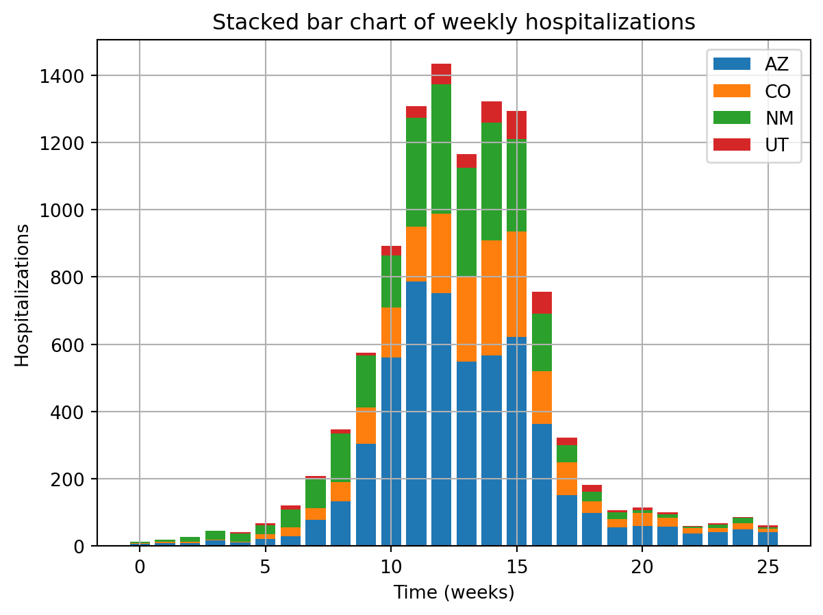

fig, axs = plt.subplots(2, 2, sharey=True)

axs = np.ravel(axs)
for i_ax in range(len(axs)):
    ax = axs[i_ax]
    ax.bar(
        time_axis,
        sim.cases[:, i_ax],
    )
    ax.set_title(f"Weekly Hosp. in {rume.scope.labels[i_ax]}")
    ax.set_xlabel("Time (weeks)")
    ax.set_ylabel("Hospitalizations")

plt.tight_layout()
plt.show()

• Run the particle filter.

output = sim.run()

• Plot the estimated beta for each state.

fig, axs = plt.subplots(2, 2, sharey=True)

key = "beta"
key_quantiles = np.array(output.param_quantiles[key])
t = np.arange(0, len(key_quantiles))

axs = np.ravel(axs)
for i_ax in range(len(axs)):
    ax = axs[i_ax]

    ax.fill_between(
        t,
        key_quantiles[:, 3, i_ax],
        key_quantiles[:, 22 - 3, i_ax],
        facecolor="blue",
        alpha=0.2,
        label="Quantile Range (10th to 90th)",
    )
    ax.fill_between(
        t,
        key_quantiles[:, 6, i_ax],
        key_quantiles[:, 22 - 6, i_ax],
        facecolor="blue",
        alpha=0.4,
        label="Quantile Range (25th to 75th)",
    )

    ax.plot(
        t,
        key_quantiles[:, 11, i_ax],
        color="red",
        label="Median (50th Percentile)",
    )

    ax.set_title(f"Estimate of '{key}' in {rume.scope.labels[i_ax]}")
    ax.set_xlabel("Time (weeks)")
    ax.set_ylabel("Quantiles")
    ax.grid(True)

plt.legend()
plt.tight_layout()
plt.show()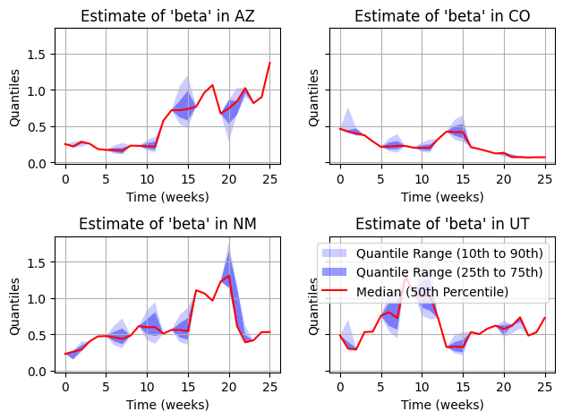

YIKES! What we see is catastrophic collapse of the particle filter. The dimentionality is too big for this type of resampler. But, we can fix this issue.

Exercise 2

The particle filter can suffer from the “curse of dimensionality”, meaning that as the number of nodes increases, the number of particles needed can increase to a point where a normal particle filter is impractical. In this case there we developed an alternative resampler called ResamplingByNode which makes a small approximation (localization technique) to greatly improve performance in multi-node systems.

• Respecify the filter type (Particle Filter) to use the ResamplingByNode.

from epymorph.parameter_fitting.utils.resampler import ResamplingByNode

filter_type = ParticleFilter(num_particles=300, resampler=ResamplingByNode)

• Create the filter simulation object.

sim = FilterSimulation(
    rume=rume,
    observations=observations,
    filter_type=filter_type,
    params_space=params_space,
)

• Run the particle filter.

output = sim.run()

• Plot the estimated beta for each state.

fig, axs = plt.subplots(2, 2, sharey=True)

key = "beta"
key_quantiles = np.array(output.param_quantiles[key])
t = np.arange(0, len(key_quantiles))

axs = np.ravel(axs)
for i_ax in range(len(axs)):
    ax = axs[i_ax]

    ax.fill_between(
        t,
        key_quantiles[:, 3, i_ax],
        key_quantiles[:, 22 - 3, i_ax],
        facecolor="blue",
        alpha=0.2,
        label="Quantile Range (10th to 90th)",
    )
    ax.fill_between(
        t,
        key_quantiles[:, 6, i_ax],
        key_quantiles[:, 22 - 6, i_ax],
        facecolor="blue",
        alpha=0.4,
        label="Quantile Range (25th to 75th)",
    )

    ax.plot(
        t,
        key_quantiles[:, 11, i_ax],
        color="red",
        label="Median (50th Percentile)",
    )

    ax.set_title(f"Estimate of '{key}' in {rume.scope.labels[i_ax]}")
    ax.set_xlabel("Time (weeks)")
    ax.set_ylabel("Quantiles")
    ax.grid(True)

plt.legend()
plt.tight_layout()
plt.show()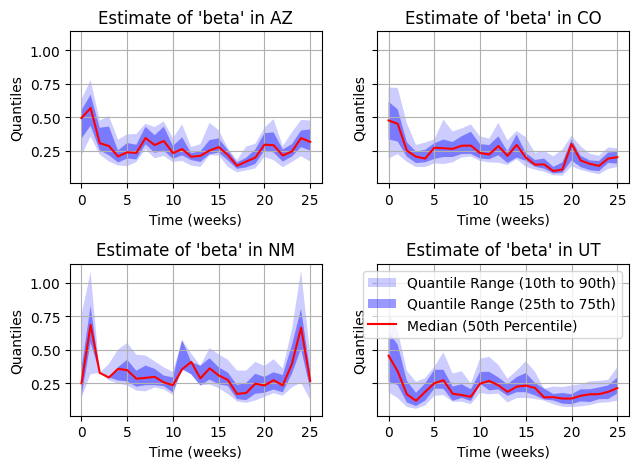

This is much better. We can still very minor issues with particle filter collapse in some areas, but in general, the estimation is much more robust. It would be recommended to increase the number of particles to make sure we don’t see any collapse.

• Plot the hospitalizations expected by the particle filter versus the true hospitalizations in each state.

fig, axs = plt.subplots(2, 2, sharey=True)

axs = np.ravel(axs)
for i_ax in range(len(axs)):
    ax = axs[i_ax]

    ax.plot(
        output.model_data[:, i_ax],
        label="Model Data",
        color="red",
        linestyle="-",
        zorder=10,
        marker="x",
    )

    ax.plot(
        output.true_data[:, i_ax],
        label="True Data",
        color="green",
        linestyle="--",
        zorder=9,
        marker="*",
    )

    ax.set_xlabel("Time (weeks)")
    ax.set_ylabel("Hospitalization")
    ax.set_title(f"Model Data vs True Data in {rume.scope.labels[i_ax]}")
    ax.grid(True)

plt.legend()
plt.tight_layout()
plt.show()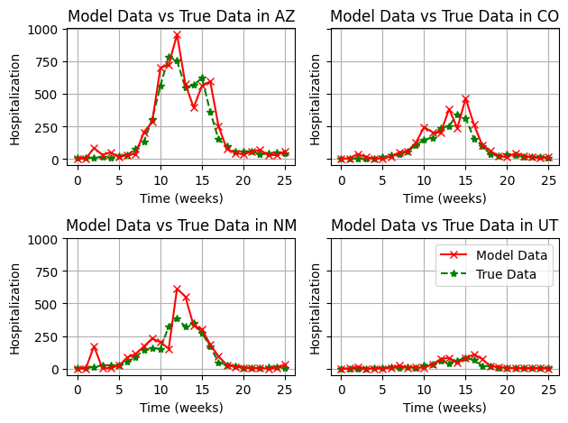

Exercise 3

In this final example, we will fit the State-specific transmission rates, but our model will also include the effects of inter-state commuter movement.

• Create a new RUME, specifying a commuter movement model.

from epymorph.adrio import commuting_flows

rume = SingleStrataRUME.build(
    ipm=ipm.SIRH(),
    mm=mm.Pei(),
    scope=StateScope.in_states(states, year=2015),
    init=Proportional(
        ratios=np.broadcast_to(
            np.array([9999, 1, 0, 0], dtype=np.int64), shape=(len(states), 4)
        )
    ),
    time_frame=TimeFrame.of("2022-09-15", 7 * 26 + 1),
    params={
        "beta": 0.3,  # Placeholder value
        "gamma": 0.2,
        "xi": 1 / 365,
        "hospitalization_prob": 200 / 100_000,
        "hospitalization_duration": 5.0,
        "population": acs5.Population(),
        "commuters": commuting_flows.Commuters(),
    },
)

Note: The commuters ADRIO takes some time to evaluate, even when the data is cached. This would be a problem if we passed this RUME directly into the particle filter, which runs hundreds of simulations. To bypass this, we’re going to precompute the commuter matrix, which is a pretty advanced technique, but saves a lot of compute time. A user could run the particle filter without this step, but it would take a lot longer to run.

• Create a copy of the RUME, but where the commuter matrix is precomputed.

import dataclasses
from epymorph.attribute import AbsoluteName, NamePattern

name = AbsoluteName(strata="gpm:all", module="mm", id="commuters")
attr_def = rume.requirements[name]

# Precompute the commuter matrix.
rng = np.random.default_rng(seed=1)
data_resolver = rume.evaluate_params(rng=rng)
commuter_matrix = data_resolver.resolve(name, attr_def)

# Create a copy of the RUME, but with the commuter matrix replaced.
params_copy = dict(rume.params)
params_copy[NamePattern.of(name.id)] = commuter_matrix
rume_copy = dataclasses.replace(rume, params=params_copy)

• We can use the same parameter space as before. However, we’ll need to create the observations object again with this new RUME declaration. Again, we use CDC weekly hospitalization data in each state.

observations = Observations(
    source=InfluenzaHospitalizationSumState(),
    model_link=ModelLink(
        quantity=rume.ipm.select.events("I->H"),
        time=rume.time_frame.select.all().group(EveryNDays(7)).agg(),
        geo=rume.scope.select.all(),
    ),
    likelihood=Poisson(),
)

• Create the filter simulation object using the RUME where we precomputed the commuter matrix.

sim = FilterSimulation(
    rume=rume_copy,
    observations=observations,
    filter_type=filter_type,
    params_space=params_space,
)

• Run the particle filter.

output = sim.run(rng=rng)

• Plot the estimated beta for each state.

fig, axs = plt.subplots(2, 2, sharey=True)

key = "beta"
key_quantiles = np.array(output.param_quantiles[key])
t = np.arange(0, len(key_quantiles))

axs = np.ravel(axs)
for i_ax in range(len(axs)):
    ax = axs[i_ax]

    ax.fill_between(
        t,
        key_quantiles[:, 3, i_ax],
        key_quantiles[:, 22 - 3, i_ax],
        facecolor="blue",
        alpha=0.2,
        label="Quantile Range (10th to 90th)",
    )
    ax.fill_between(
        t,
        key_quantiles[:, 6, i_ax],
        key_quantiles[:, 22 - 6, i_ax],
        facecolor="blue",
        alpha=0.4,
        label="Quantile Range (25th to 75th)",
    )

    ax.plot(
        t,
        key_quantiles[:, 11, i_ax],
        color="red",
        label="Median (50th Percentile)",
    )

    ax.set_title(f"Estimate of '{key}' in {rume.scope.labels[i_ax]}")
    ax.set_xlabel("Time (weeks)")
    ax.set_ylabel("Quantiles")
    ax.grid(True)

plt.legend()
plt.tight_layout()
plt.show()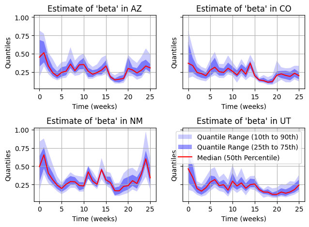

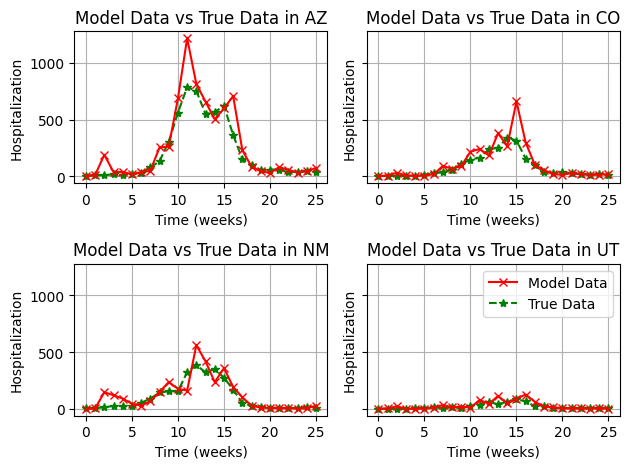
We can see that the estimates of transmission rate are not very different, such that movement at this spatial scale (State-level) likely does not have a huge effect on the local and regional dynamics.

• Plot the hospitalizations expected by the particle filter versus the true hospitalizations in each state.

fig, axs = plt.subplots(2, 2, sharey=True)

axs = np.ravel(axs)
for i_ax in range(len(axs)):
    ax = axs[i_ax]

    ax.plot(
        output.model_data[:, i_ax],
        label="Model Data",
        color="red",
        linestyle="-",
        zorder=10,
        marker="x",
    )

    ax.plot(
        output.true_data[:, i_ax],
        label="True Data",
        color="green",
        linestyle="--",
        zorder=9,
        marker="*",
    )

    ax.set_xlabel("Time (weeks)")
    ax.set_ylabel("Hospitalization")
    ax.set_title(f"Model Data vs True Data in {rume.scope.labels[i_ax]}")
    ax.grid(True)

plt.legend()
plt.tight_layout()
plt.show()