Multi-node Simulations with Movement Models

SCENARIO:

Imagine a new respiratory pathogen emerges in Maricopa County, AZ where 5 people are initially infected. In an effort to control the outbreak, local public health officials across the state have asked us for guidance on how the pathogen might spread to different counties. We therefore need to consider human movement patterns in our model to understand spatial spread. We will build a County-level spatial model with epymorph, such that each node of our model represents the population in a single county. The model then assumes that the populations within the county interact homogeneously. Each node is interconnected through human movement, which affects the regional spread of the pathogen.

The exercises in this vignette show you how to add nodes and movement between nodes to your disease models in epymorph and will explore how varying how we model movement (i.e., the assumptions that govern movement flows) might impact disease dynamics.

Exercise 1

• Put your necessary imports here for setting up the simulations.

import matplotlib.pyplot as plt
import numpy as np

from epymorph.kit import *
from epymorph.adrio import acs5

• Build a County Scope for Arizona. Print the node labels to see the county names.

my_scope = CountyScope.in_states(['AZ'], year=2020)
my_scope.labels
# You can also see their FIPS code:
# my_scope.node_ids

array(['Apache, AZ', 'Cochise, AZ', 'Coconino, AZ', 'Gila, AZ',
       'Graham, AZ', 'Greenlee, AZ', 'La Paz, AZ', 'Maricopa, AZ',
       'Mohave, AZ', 'Navajo, AZ', 'Pima, AZ', 'Pinal, AZ',
       'Santa Cruz, AZ', 'Yavapai, AZ', 'Yuma, AZ'], dtype='<U14')

• For your IPM, import the SIRS model from the epymorph library and plot the diagram.

from epymorph.data.ipm.sirs import SIRS
sirs_ipm = SIRS()

sirs_ipm.diagram()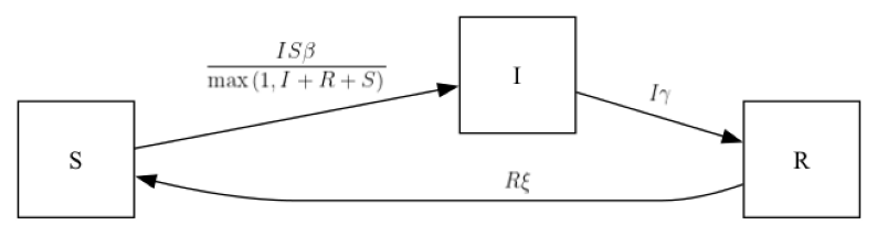

• Select your movement model by importing the movement model from the epymorph library called ‘Flat’. This movement model includes random movement to and from a node. In other words, any individual has an equal chance of moving to any other node in the system per time step. However, this model assumes individuals do not necessarily return to their original node.

from epymorph.data.mm.flat import Flat
flat_mm = Flat()

• Initialize the state variables in our model (i.e., the initial values of S, I, and R). In this scenario, the infection began in Maricopa County, Arizona with 5 infected individuals.

# Maricopa is the 8th node in the scope (i.e., index 7)
my_init = init.SingleLocation(location=7, seed_size=5)

• Define your timeframe.

time = TimeFrame.of("2020-01-01", duration_days=190)

• Define a parameter that is required by the Flat movement model, called commuter_proportion. This represents the fraction of individuals in a given node that move outside their node on a daily basis.

comm_prop = 0.15

• Define the model parameters, ‘beta’ (transmission rate), ‘gamma’ (recovery rate), and ‘xi’ (latency rate) to reasonable values.

beta = 0.4
gam = 1 / 4
xi = 1 / 200

• Construct the RUME from your various requirements.

rume = SingleStrataRUME.build(
    scope=my_scope,
    ipm=sirs_ipm,
    mm=flat_mm,
    init=my_init,
    time_frame=time,
    params={
        'beta': beta,
        'gamma': gam,
        'xi': xi,
        'population': acs5.Population(),
        'commuter_proportion': comm_prop,
    }
)
# Print a description of params
print(rume.params_description())

ipm::beta (type: float, shape: TxN)
    infectivity

ipm::gamma (type: float, shape: TxN)
    progression from infected to recovered

ipm::xi (type: float, shape: TxN)
    progression from recovered to susceptible

mm::population (type: int, shape: N)
    The total population at each node.

mm::commuter_proportion (type: float, shape: S, default: 0.1)
    The proportion of the total population which commutes.

init::population (type: int, shape: N)
    The population at each geo node.

• Run your simulation

sim = BasicSimulator(rume)
with sim_messaging(live = False):
    out = sim.run(
        rng_factory=default_rng(5),
    )

Loading gpm:all::mm::population (epymorph.adrio.acs5.Population):
  |####################| 100%  (1.055s)
Running simulation (BasicSimulator):
• 2020-01-01 to 2020-07-08 (190 days)
• 15 geo nodes
  |####################| 100% 
Runtime: 0.903s

• Plot the dynamics of the Infectious class over time as a single line for each county and explore the differences in peak infection for each county. You’ll want to group by ‘day’ to aggregate across the time ticks in the model imposed by the movement model.

out.plot.line(
    geo=out.rume.scope.select.all(),
    time=out.rume.time_frame.select.all().group("day").agg(),
    quantity=out.rume.ipm.select.compartments("I"),
    title="Infectious in AZ Counties",
    legend="outside",
)

• Use the quantile table feature to print the maximum infectious observed across the counties.

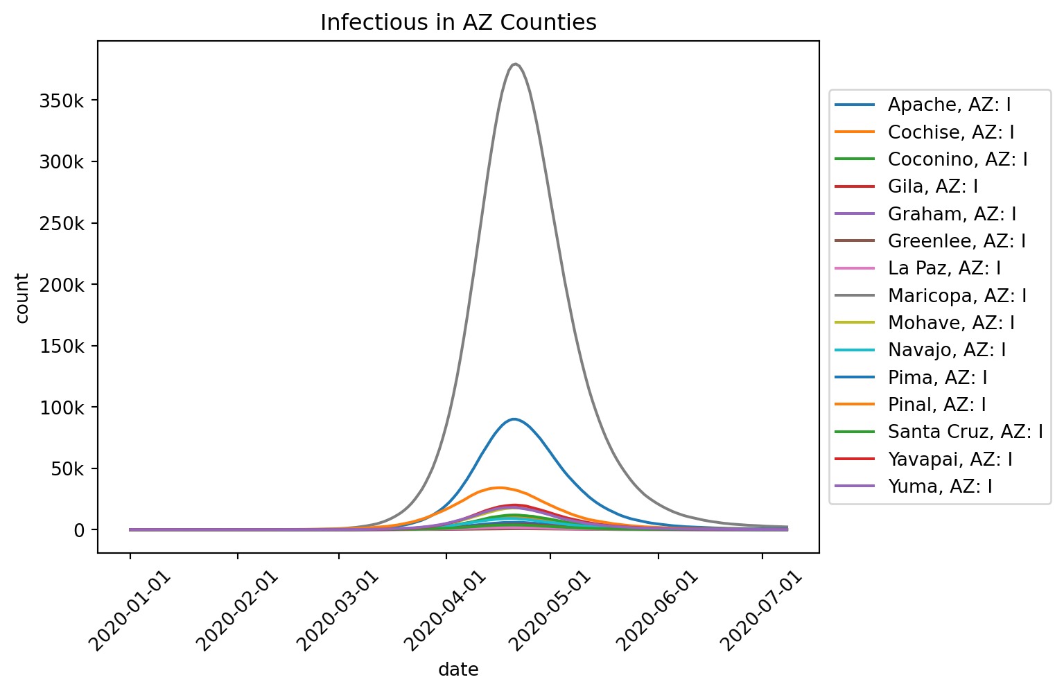
out.table.quantiles(
    quantiles=[1.0],
    geo=out.rume.scope.select.all(),
    time=out.rume.time_frame.select.all().group("day").agg(),
    quantity=out.rume.ipm.select.compartments("I"),
)

	geo	quantity	1.0
0	Apache, AZ	I	5990.0
1	Cochise, AZ	I	10481.0
2	Coconino, AZ	I	11939.0
3	Gila, AZ	I	4234.0
4	Graham, AZ	I	3259.0
5	Greenlee, AZ	I	767.0
6	La Paz, AZ	I	1855.0
7	Maricopa, AZ	I	379413.0
8	Mohave, AZ	I	17673.0
9	Navajo, AZ	I	9060.0
10	Pima, AZ	I	90031.0
11	Pinal, AZ	I	34140.0
12	Santa Cruz, AZ	I	3875.0
13	Yavapai, AZ	I	20063.0
14	Yuma, AZ	I	18073.0

• Create a map that shows the maximum infectious in each county, in the time interval nearest to the peak. Transform with a log10 scale.

def log10_transform(data_df):
    # we have to be careful to avoid log(0)!
    log_value = data_df["data"].apply(lambda x: np.log10(x) if x > 0 else nan)
    return data_df.assign(data=log_value)

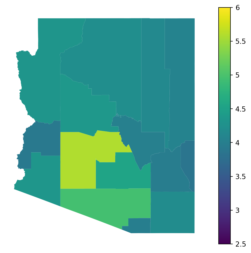
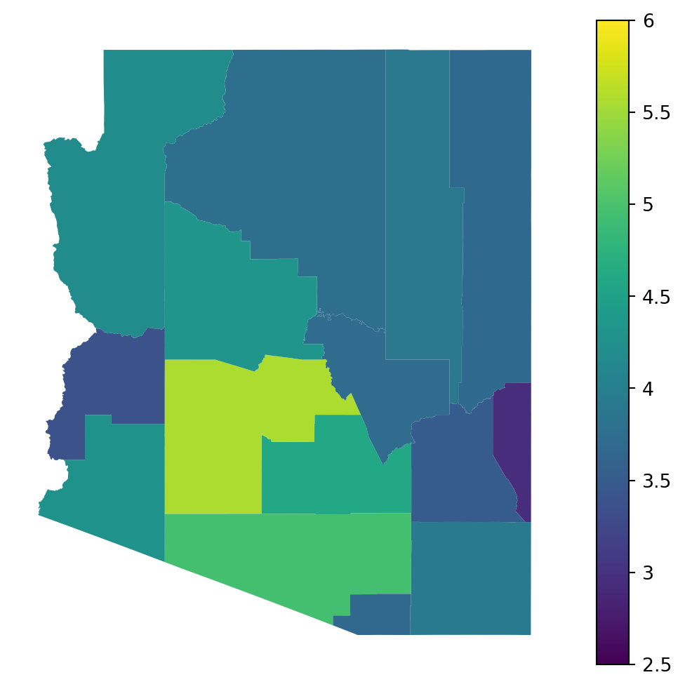
out.map.choropleth(
    geo=rume.scope.select.all(),
    time=rume.time_frame.select.rangex("2020-04-01", "2020-05-01").agg(compartments="max"),
    quantity=rume.ipm.select.compartments("I"),
    transform=log10_transform,
    vmax = 6.0,
    vmin = 2.5,
)

Exercise 2

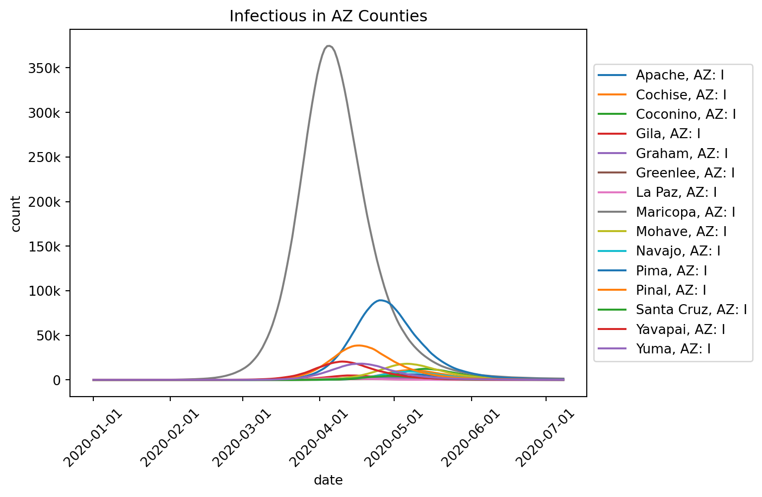
In Exercise 1, we used a “flat” movement model, in which individuals could move equally randomly to any other node. This led to more or less syncronous outbreaks across space, which is of course not very realistic. In this Exercise, we’ll use more realistic movement models.

• Create a new RUME, but using the Centroids movement model. This movement model assumes that the probability of moving between nodes in the scope is defined by a distance-based probability kernel.

Note that this new MM requires a calculation of centroids, but this can be done using the us_tiger ADRIO. Additionally, we need a parameter ‘phi’ which modulates the effect of distance in the probability kernel. On your own, you can test how ‘phi’ influences the dynamics.

from epymorph.data.mm.centroids import Centroids
from epymorph.adrio import us_tiger

rume = SingleStrataRUME.build(
    scope=my_scope,
    ipm=sirs_ipm,
    mm=Centroids(),
    init=my_init,
    time_frame=time,
    params={
        #For IPM
        'beta': beta,
        'gamma': gam,
        'xi': xi,
        #For MM
        'population': acs5.Population(),
        'commuter_proportion': comm_prop,
        'centroid': us_tiger.InternalPoint(),
        'phi': 20.0,
    }
)

print(rume.params_description())

ipm::beta (type: float, shape: TxN)
    infectivity

ipm::gamma (type: float, shape: TxN)
    progression from infected to recovered

ipm::xi (type: float, shape: TxN)
    progression from recovered to susceptible

mm::population (type: int, shape: N)
    The total population at each node.

mm::centroid (type: [(longitude, float), (latitude, float)], shape: N)
    The centroids for each node as (longitude, latitude) tuples.

mm::phi (type: float, shape: S, default: 40.0)
    Influences the distance that movers tend to travel.

mm::commuter_proportion (type: float, shape: S, default: 0.1)
    The proportion of the total population which commutes.

init::population (type: int, shape: N)
    The population at each geo node.

sim = BasicSimulator(rume)
with sim_messaging(live = False):
    out = sim.run(
        rng_factory=default_rng(5),
    )

Loading gpm:all::mm::population (epymorph.adrio.acs5.Population):
  |####################| 100%  (0.579s)
Loading gpm:all::mm::centroid (epymorph.adrio.us_tiger.InternalPoint):
  |####################| 100%  (0.704s)
Running simulation (BasicSimulator):
• 2020-01-01 to 2020-07-08 (190 days)
• 15 geo nodes
  |####################| 100% 
Runtime: 0.807s

• Again, plot the dynamics of the Infectious class over time as a single line for each county and explore the differences in peak infection for each county. Now you should see a more marked delay in the pathogen spreading from county to county.

out.plot.line(
    geo=out.rume.scope.select.all(),
    time=out.rume.time_frame.select.all().group("day").agg(),
    quantity=out.rume.ipm.select.compartments("I"),
    title="Infectious in AZ Counties",
    legend="outside",
)

• Again, create a map that shows the maximum infectious in each county, and use the same time frame as in Exercise 1. Transform with a log10 scale. You should notice a marked change, indicating that the time of the peak has substantially shifted due to different movement dynamics.

out.map.choropleth(
    geo=rume.scope.select.all(),
    time=rume.time_frame.select.rangex("2020-04-01", "2020-05-01").agg(compartments="max"),
    quantity=rume.ipm.select.compartments("I"),
    transform=log10_transform,
    vmax = 6.0,
    vmin = 2.5,
)

Exercise 3

Finally, use a movement model that is based on real data on human behavior. Specifically, we will use a commuter-style movement model created from a model published by Pei et al. This model requires a commuter matrix, and we will use mobility data from the ACS5 commuting flows, which are at the County level. Notice that for the MM, we will use some control parameters with their defaults.

from epymorph.data.mm.pei import Pei as CommuterMM
from epymorph.adrio import commuting_flows 


rume = SingleStrataRUME.build(
    scope=my_scope,
    ipm=sirs_ipm,
    mm=CommuterMM(),
    init=my_init,
    time_frame=time,
    params={
        #For IPM
        'beta': beta,
        'gamma': gam,
        'xi': xi,
        #For MM
        'commuters': commuting_flows.Commuters(),
        # General:
        'population': acs5.Population(),
    }
)

print(rume.params_description())

ipm::beta (type: float, shape: TxN)
    infectivity

ipm::gamma (type: float, shape: TxN)
    progression from infected to recovered

ipm::xi (type: float, shape: TxN)
    progression from recovered to susceptible

mm::commuters (type: int, shape: NxN)
    A node-to-node commuters marix.

mm::move_control (type: float, shape: S, default: 0.9)
    A factor which modulates the number of commuters by conducting a
    binomial draw with this probability and the expected commuters
    from the commuters matrix.

mm::theta (type: float, shape: S, default: 0.1)
    A factor which allows for randomized movement by conducting a
    poisson draw with this factor times the average number of
    commuters between two nodes from the commuters matrix.

init::population (type: int, shape: N)
    The population at each geo node.

sim = BasicSimulator(rume)
with sim_messaging(live = False):
    out = sim.run(
        rng_factory=default_rng(5),
    )

Loading gpm:all::mm::commuters (epymorph.adrio.commuting_flows.Commuters):
  |####################| 100%  (10.932s)
Loading gpm:all::init::population (epymorph.adrio.acs5.Population):
  |####################| 100%  (0.628s)
Running simulation (BasicSimulator):
• 2020-01-01 to 2020-07-08 (190 days)
• 15 geo nodes
  |####################| 100% 
Runtime: 0.983s

• Again, plot the dynamics of the Infectious class over time as a single line for each county and explore the differences in peak infection for each county. The difference due to the more realistic movement model should be noted.

out.plot.line(
    geo=out.rume.scope.select.all(),
    time=out.rume.time_frame.select.all().group("day").agg(),
    quantity=out.rume.ipm.select.compartments("I"),
    title="Infectious in AZ Counties",
    legend="outside",
)