Seasonality Beta Editing

SCENARIO:

In many modeling scenarios, it is important to account for seasonal changes in the transmission rate of a pathogen. A classic example is measles, which typically circulates amongst school-aged children. Transmission rate is assumed to be higher during the academic year, but lower in the summer months, when there is less indoor contact between school-aged children. We can address this issue by assuming a time-varying rate of transmission in the model. The exercises in this vignette show you how to do this in epymorph, as well as exploring how seasonally-changing transmission rates can lead to stable cycling of a disease.

Exercise

• Create a classic SIRS IPM.

import matplotlib.pyplot as plt
import numpy as np
from sympy import Max

from epymorph.kit import *
from epymorph.adrio import acs5

class SIRS(CompartmentModel):
    """Defines a compartmental IPM for a generic SIR model."""
    compartments = [
        compartment('S'),
        compartment('I'),
        compartment('R'),
    ]

    requirements = [
        AttributeDef('beta', type=float, shape=Shapes.TxN,
                     comment='infectivity'),
        AttributeDef('gamma', type=float, shape=Shapes.TxN,
                     comment='recovery rate'),
        AttributeDef('latent', type=float, shape=Shapes.TxN,
                     comment='recovery rate'),
    ]

    def edges(self, symbols):
        [S, I, R] = symbols.all_compartments
        [β, γ, l] = symbols.all_requirements

        N = Max(1, S + I + R)

        return [
            edge(S, I, rate=β * S * I / N),
            edge(I, R, rate=γ * I),
            edge(R, S, rate=l * R),
        ]

• Model the transmission rate as a step function. Specifically, assume that the transmission rate increases during the academic year, but decreases during the middle of the year (i.e., summer months). This will require you to create a class function to calculate the transmission rate as a function of time.

class Step_Beta(ParamFunctionTimeAndNode):

    def evaluate1(self, day: int, node_index: int) -> float:
        winter_beta = 1.0
        summer_beta = 0.5
        summer_start = 120
        summer_end = 221
        t_mod = day % 365

        if summer_start <= t_mod <= summer_end:
            x = summer_beta

        else:
            x = winter_beta

        return x

• Build a county-level RUME.

scope = CountyScope.in_counties(['Maricopa, AZ'], year=2020)
my_ipm = SIRS()
null_mm = mm.No()

rume = SingleStrataRUME.build(
    ipm=my_ipm,
    mm=null_mm,
    init=init.SingleLocation(location=0, seed_size=5),
    scope=scope,
    time_frame=TimeFrame.of("2015-01-01", 365 * 3),
    params={
        'beta': Step_Beta(),
        'gamma': 1 / 3,
        'latent': 1 / 120,
        'population': acs5.Population(),
    }
)

• Before you run a simulation of the RUME, generate a plot that shows the expected value of transmission rate over time, based on your sinusoidal function. You will evaluate the value of the parameter in context of the RUME you specified.

# Evaluate the transmission rates
beta_values = (
    Step_Beta()
    .with_context(
        scope=rume.scope,
        time_frame=rume.time_frame,
    )
    .evaluate()
)

### GRAPH ###
fig, ax = plt.subplots()
ax.plot(beta_values)
ax.set(title="beta function", ylabel="beta", xlabel="days")
fig.tight_layout()
plt.show()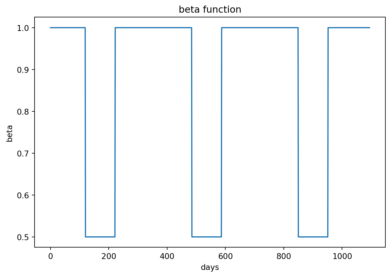

• Run a simulation of the RUME, and plot the compartment values over time. You should see stable cycling due to waning immunity and seasonal forcing.

sim = BasicSimulator(rume)
with sim_messaging(live = False):
    out = sim.run(
        rng_factory=default_rng(5),
    )

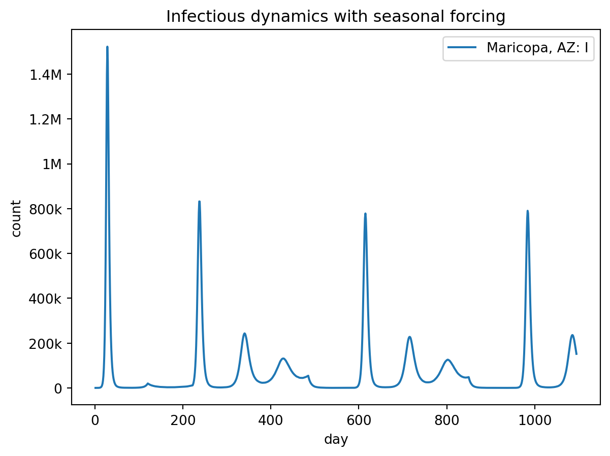
out.plot.line(
    geo=out.rume.scope.select.all(),
    time=out.rume.time_frame.select.all(),
    quantity=out.rume.ipm.select.compartments("I"),
    title="Infectious dynamics with seasonal forcing",
)

Loading gpm:all::init::population (epymorph.adrio.acs5.Population):
  |####################| 100%  (0.691s)
Running simulation (BasicSimulator):
• 2015-01-01 to 2017-12-30 (1095 days)
• 1 geo nodes
  |####################| 100% 
Runtime: 0.218s