Birth-death IPM modeling example

SCENARIO:

In many modeling scenarios, it is important to account for changes in host populations over time due to births and deaths. In some cases, losses may be due to fatalities due to pathogen infection; in other scenarios, the organisms being modeled simply have natural life spans or cycles that fall within the modeling timeframe. In either case, we address this issue by adding explicit “birth” and “death” compartments to our model. The exercises in this vignette show you how to do this in epymorph, as well as exploring how birth/death dynamics can affect model behavior.

Exercise 1

Put your necessary imports here for setting up the simulations and graphs

import matplotlib.pyplot as plt
import numpy as np
from sympy import Max

from epymorph.kit import *
from epymorph.adrio import acs5

Copy the basic SIR model from the epymorph library and alter it to create a new model of SIR with host demography. First, add the special compartment called “BIRTH” to your model. To do this, add a new edge connecting the ‘BIRTH’ compartment to the ‘S’ compartment, using the the rate equation “birth_rate * N”. This assumes that all hosts can have offspring, and all of those offspring will be susceptible.

Then, add the special compartment called “DEATH” to your model adding several edges from S, I, and R to “DEATH” with a rate of “death_rate*[State Variable]”. It is simplest to assume that birth_rate and death_rate are equivalent.

Note that the model also includes wanining immunity.

class BSIRD_ipm(CompartmentModel):
    compartments = [
        compartment("S"),
        compartment("I"),
        compartment("R"),
    ]
    requirements = [
        AttributeDef("beta", type=float, shape=Shapes.TxN, comment="infectivity"),
        AttributeDef(
            "gamma",
            type=float,
            shape=Shapes.TxN,
            comment="progression from infected to recovered",
        ),
        AttributeDef(
            "xi",
            type=float,
            shape=Shapes.TxN,
            comment="progression from recovered to susceptible",
        ),
        AttributeDef(
            "birth_rate",
            type=float,
            shape=Shapes.TxN,
            comment="birth rate per day per capita",
        ),
        AttributeDef(
            "death_rate",
            type=float,
            shape=Shapes.TxN,
            comment="death rate per day per capita",
        ),
    ]

    def edges(self, symbols):
        [S, I, R] = symbols.all_compartments
        [β, γ, ξ, br, dr] = symbols.all_requirements

        N = Max(1, S + I + R)

        return [
            # traditional formulation for S,I,R
            edge(S, I, rate=β * S * I / N),
            edge(I, R, rate=γ * I),
            edge(R, S, rate=ξ * R),
            # newborn individuals enter S
            edge(BIRTH, S, rate=br * (S + I + R)),
            # death edges
            edge(S, DEATH, rate=dr * S),
            edge(I, DEATH, rate=dr * I),
            edge(R, DEATH, rate=dr * R),
        ]

Exercise 2

Use epymorph’s built-in feature to plot your model diagram (i.e., the box-and-arrow flow diagram of the system of equations).

my_ipm = BSIRD_ipm()
my_ipm.diagram()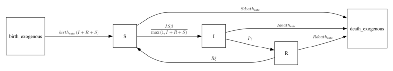

The SIR model with demography, box-and-arrow diagram.

Choose a single node GEO and null MM. You’ll need a very large population size to see how this model works over the long term. We suggest running the model for a few years. Based on the suggested parameter values, shown below, you should see damped oscillation dynamics.

scope = CountyScope.in_counties(["04013"], year=2020)  # Maricopa County
time = TimeFrame.of("2020-01-01", 365 * 3)
null_mm = mm.No()

Initialize the system with 5 infected individuals.

my_init = init.SingleLocation(location=0, seed_size=5)

Create the RUME and run your simulation. Our example gives reasonable parameter values.

rume = SingleStrataRUME.build(
    ipm=BSIRD_ipm(),
    mm=null_mm,
    init=my_init,
    scope=scope,
    time_frame=time,
    params={
        "beta": 0.4,
        "gamma": 1 / 4,
        "xi": 1 / 120,
        "birth_rate": 1 / (70 * 365),
        "death_rate": 1 / (70 * 365),
        "population": acs5.Population(),
    },
)

sim = BasicSimulator(rume)
with sim_messaging(live = False):
    out = sim.run(
        rng_factory=default_rng(5),
    )

Loading gpm:all::init::population (epymorph.adrio.acs5.Population):
  |####################| 100%  (1.028s)
Running simulation (BasicSimulator):
• 2020-01-01 to 2022-12-30 (1095 days)
• 1 geo nodes
  |####################| 100% 
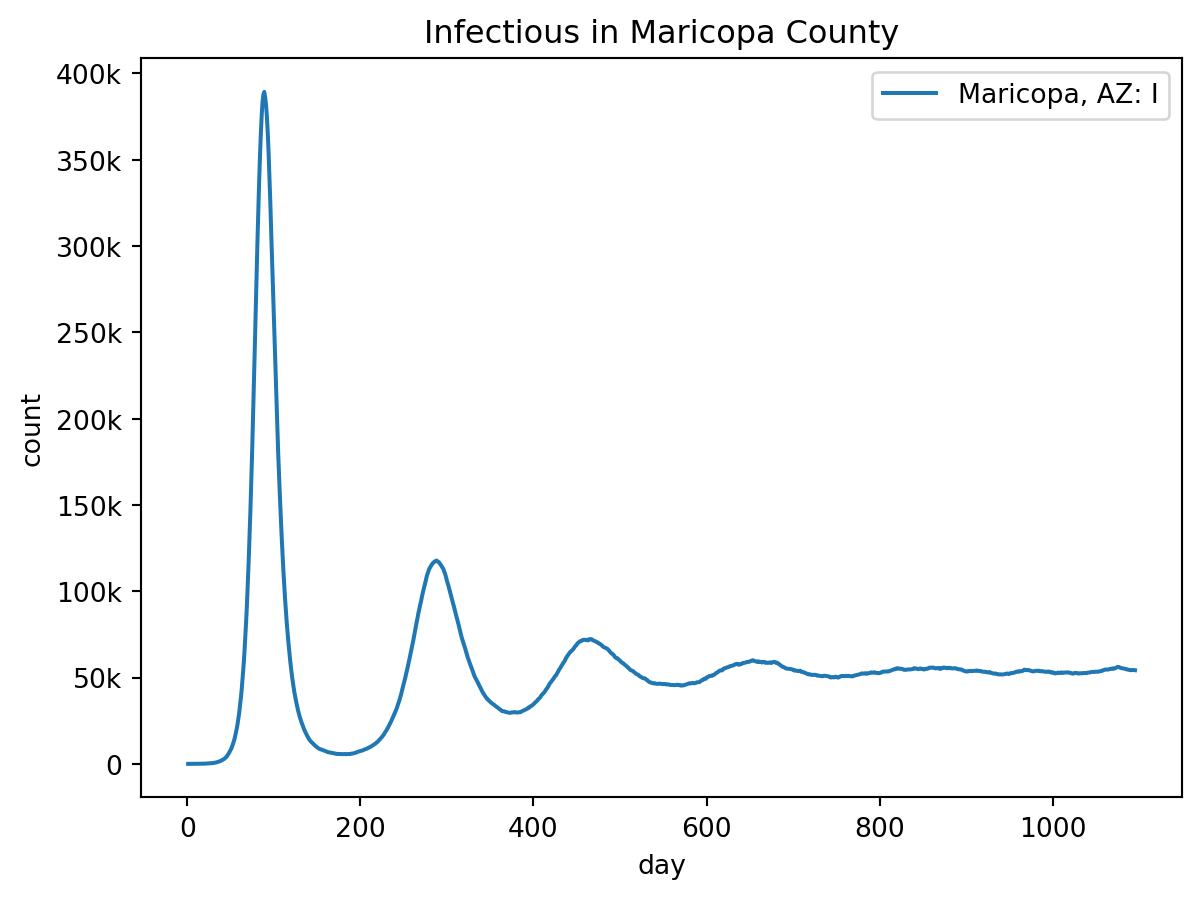
Runtime: 0.284s

Plot the dynamics of the Infectious class over time. Note that you may need to run your model with a different random seed, in case early burnout occurs.

out.plot.line(
    geo=out.rume.scope.select.all(),
    time=out.rume.time_frame.select.all(),
    quantity=out.rume.ipm.select.compartments("I"),
    title="Infectious in Maricopa County",
)

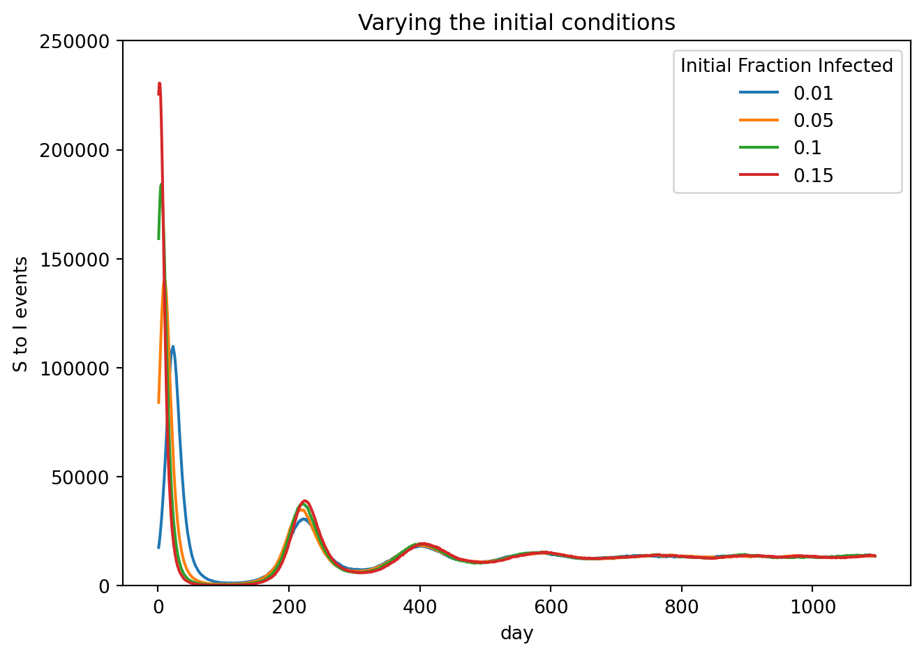
Exercise 3

ADVANCED: Basic epi theory shows that this model leads to a stable point equilibrium where the dynamics proceed to this stable point with damped oscillations. Set up an array of initial conditions (i.e., different fractions of the population initially infected), and run your simulation for each initial condition. Plot all of the Infectious over time curves on the same graph to show that even if the model starts with fractions of the population initially infected, the model goes to the same stable point.

stored_sim_results = []
initial = [0.01, 0.05, 0.10, 0.15]

for frac in initial:
    rume = SingleStrataRUME.build(
        ipm=BSIRD_ipm(),
        mm=null_mm,
        init=init.Proportional(ratios=np.array([1 - frac, frac, 0])),
        scope=scope,
        time_frame=time,
        params={
            "beta": 0.4,
            "gamma": 1 / 4,
            "xi": 1 / 120,
            "birth_rate": 1 / (70 * 365),
            "death_rate": 1 / (70 * 365),
            "population": acs5.Population(),
        },
    )
    sim = BasicSimulator(rume)
    out = sim.run(
        rng_factory=default_rng(5),
    )
    stored_sim_results.append(out)

fig, ax = plt.subplots()

for j in stored_sim_results:
    j.plot.line_plt(
        ax = ax,
        geo=j.rume.scope.select.all(),
        time=j.rume.time_frame.select.all(),
        quantity=j.rume.ipm.select.events("S->I"),
    )

ax.set_ylim(bottom=0,top=2.5e5)
ax.set_xlabel("day")
ax.set_ylabel("S to I events")
ax.set_title("Varying the initial conditions")
ax.grid(False)
plt.legend(initial, title="Initial Fraction Infected")
fig.tight_layout()
plt.show()